Normalizing Data - Part 1 of AI Series

Co-authored by Naveen (AI Dev at Skcript).

In Machine Learning, more often than not applying an algorithm to data is not hard, rather representing the data usually is. But sometimes representing data a certain way works for one algorithm, but completely implodes for another. So with all these variations, is there one compartmentalized approach to follow?

Yes! (well, kind of and ‘kind of’ in ML is ‘good enough’)

Normalization

The boring definition of this mathematical approach would be,

Normalization is performed on data to remove amplitude variation and only focus on the underlying distribution shape.

Well, who does that make sense to? To put normalization in perspective, it can be defined as,

Normalization is performed on data to compare numeric values obtained from different scales.

Source: https://www.utdallas.edu/~herve/abdi-Normalizing2010-pretty.pdf

Why do we normalize?

Simply put, how do we compare a score 8 in a singing competition to a score of 100 in an I.Q. test? In order to do so, we need to “eliminate” the unit of measurement, and this operation is called normalizing the data.

So, normalization brings any dataset to a comparable range. It could be to squash down the data to fit between the range of [0,1] or [-1,1] or anything else!

Alright, so we know why we need normalization, but when do we use it?

When do we normalize?

In basic terms you need to normalize data when the algorithm predicts based on the weighted relationships formed between data points.

For example if you had a dataset that predicts the onset of diabetes where your data points are glucose levels and age, and your algorithm is PCA, you would need to normalize!

Why? Because, PCA predicts by maximizing the variance. Here, the glucose levels data point would vary in decimal points, but age would only differ by integer values. To bring them both to scale, use normalization! You can now compare glucose levels and age, even if they were initially meaningless.

However, if you were to use a decision tree, normalization wouldn’t really matter, since it compares each data point to itself and not to any other data point.

Normalization Methods

I’m picking Python to show you how normalization affects data. We will be using the numpy and scikit-learn packages to perform the operations. Normalization will be performed on this dataset.

1. Min Max Normalization

Min Max Normalization transforms a value A to B which fits in the range [C,D]. We can do this by applying the formula below,

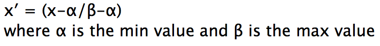
This ensures that no matter what scale your data is in, it will be converted to fall between the range of 0 to 1.

import numpy as np
from sklearn.preprocessing import minmax_scale

minmax_scale(np.array([1,2,3,4,5]))
=> array([ 0.  ,  0.25,  0.5 ,  0.75,  1.  ])

To see Min Max used on a real dataset, check this repo.

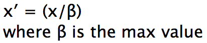
2. Max Normalization

Max is quite similar to Min Max normalization. The only difference being is that the the normalized values will fall between a range of 1 and to a value less than or equal to 0.

import numpy as np
from sklearn.preprocessing import normalize

normalize(np.array([1,2,3,4,5]).reshape(1, -1), norm="max")
=> array([[ 0.2,  0.4,  0.6,  0.8,  1. ]])

To see Max used on a real dataset, check this repo.

3. L1 Normalization (Least Absolute Deviation or LAD)

L1 is basically minimizing the sum of the absolute differences (S) between the target value (x) and the estimated values (x’).

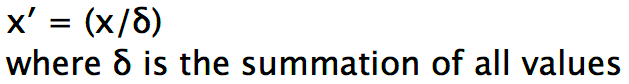
To understand it easily, its just adding all the values in the array and dividing each of it using the sum.

import numpy as np
from sklearn.preprocessing import normalize

normalize(np.array([1,2,3,4,5]).reshape(1, -1), norm="l1")
=> array([[ 0.06666667,  0.13333333,  0.2       ,  0.26666667,  0.33333333]])

To see L1 used on a real dataset, check this repo.

4. L2 Normalization (Least Square Error or LSE)

L2 minimizes the sum of the square of the differences (S) between the target value (x) and the estimated values (x’).

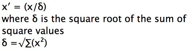
Or in simpler terms, just divide each value by δ. Where δ is nothing but the square root of the sum of all the squared values.

import numpy as np
from sklearn.preprocessing import normalize

normalize(np.array([1,2,3,4,5]).reshape(1, -1), norm="l2")
=> array([[ 0.13483997,  0.26967994,  0.40451992,  0.53935989,  0.67419986]])

To see L2 used on a real dataset, check this repo.

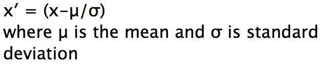
5. Z-Score

Simply put, a z-score is the number of standard deviations from the mean a data point is. But more technically it’s a measure of how many standard deviations below or above the dataset mean a datapoint is. A z-score is also known as a standard score and it can be placed on a normal distribution curve.

Z-scores range from -3 standard deviations (which would fall to the far left of the normal distribution curve) up to +3 standard deviations (which would fall to the far right of the normal distribution curve).

In order to use a z-score, you need to know the mean μ and also the population standard deviation σ.

Z-scores are a way to compare results from a test to a “normal” population. Results from tests or surveys have thousands of possible results and units. However, those results can often seem meaningless.

For example, knowing that someone’s weight is 150 pounds might be good information, but if you want to compare it to the “average” person’s weight, looking at a vast table of data can be overwhelming (especially if some weights are recorded in kilograms). A z-score can tell you where that person’s weight is compared to the average population’s mean weight.

For a complete implementation of Z-Score please have a look at this repo.